Adaptive retrieval and shortening embeddings
OpenAI latest embedding models support shortening embeddings, where developers could simply “remove some numbers from the end of a sequence” and still maintain a valid representation for text.
This enables very flexible usage. For example, when using a vector data store that only supports embeddings up to 1024 dimensions long, developers can now still use our best embedding model text-embedding-3-large and specify a value of 1024 for the dimensions API parameter, which will shorten the embedding down from 3072 dimensions, trading off some accuracy in exchange for the smaller vector size.
Shortening embeddings
OpenAI's new embedding model text-embedding-3-large produces embeddings with 3072 dimensions by default.

But you could safely remove some numbers from the end of the sequence and still maintain a valid representation for text. For example, you could shorten the embeddings to 1024 dimensions.
Details
You may need normalization to ensure that the shortened embeddings compatible with some distance calculation e.g. dot poroduct. OpenAI's API will help you on this if you are calling text-embedding-3-large to generate a lower dimension embedding directly, instead of truncating the original embeddings on your own.
embedding_3072_dim_from_openai = [-0.00611, -0.00269, ...]
embedding_1024_dim_from_openai = [-0.01520, -0.03839, ...]

embedding_1024_dim_truncated_from_3072_dim = [-0.00611, -0.00269, ...]
embedding_1024_dim_normalized = [-0.01520, -0.03839, ...]
There are lots of benefits to using shortening embeddings:
- Reduced memory usage: Shortening embeddings can reduce the memory usage to store the embeddings.
- Lower dimensions: Shortening embeddings can reduce the dimensions of the embeddings. Some vector data stores only support embeddings up to a certain number of dimensions (e.g. 2000).
- Faster indexing and search: Smaller embeddings can be indexed and searched faster than larger embeddings.
- Trade-off performance and cost: Shortening embeddings can trade off some accuracy in exchange for the smaller vector size.
However, the accuracy of the shortened embeddings is not as good as the full embeddings.
Trade-off performance and cost
We have performed an experiment to evaluate the effectiveness of reduced embeddings compared to the complete embeddings. The benchmark was conducted using the dbpedia-entities-openai3-text-embedding-3-large-3072-1M dataset. The experiment was carried out on a Google Cloud VM with specifications of n2-standard-8, which includes 8 vCPUs and 32 GB of memory.
We have established a table and populated it with 1 million embeddings, each consisting of 3072 dimensions.
CREATE TABLE openai3072 (
  id bigserial PRIMARY KEY,
  text_embedding_3_large_3072_embedding vector(3072),
  text_embedding_3_large_3072_embedding bvector(3072)
);
Details
The code for inserting 1M embeddings into the table:
from pgvecto_rs.sdk import PGVectoRs, Record
from pgvecto_rs.psycopg import register_vector
import psycopg

conn = psycopg.connect(conninfo='postgresql://postgres:mysecretpassword@localhost:5433/postgres', autocommit=True)

import json
import os

import numpy as np
import random
from datasets import load_dataset
from datasets.exceptions import DatasetNotFoundError
from tqdm import tqdm

MODEL_NAME, DIMENSIONS = "text-embedding-3-large", 3072
DATASET_NAME = f"Qdrant/dbpedia-entities-openai3-{MODEL_NAME}-{DIMENSIONS}-1M"
collection_name = f"dbpedia-{MODEL_NAME}-{DIMENSIONS}"
embedding_column_name = f"{MODEL_NAME}-{DIMENSIONS}-embedding"

dataset = load_dataset(
        DATASET_NAME,
        streaming=False,
        split="train",
    )

bs = 1000
for i, record in tqdm(enumerate(dataset)):
    if i % bs == 0:
        points = []
    points.append({
        "embedding": record[embedding_column_name]
    })
    if i % bs == bs - 1:
        batch_points = f", ".join([f"('{p['embedding']}')" for p in points])
        conn.execute(f"INSERT INTO openai3072 (text_embedding_3_large_3072_embedding) VALUES %s" % (batch_points))
    print(f"Inserted {i} records")
Furthermore, we have created indexes for embeddings with dimensions of 256, 1024 and 3072, and performed an ANN (Approximate Nearest Neighbors) query for each dimension. There is no need to create the 256-dimensional column, as we can use the first 256 dimensions of the 3072-dimensional embeddings.
-- Create 256-dim index
CREATE INDEX openai_vector_index_256 ON public.openai3072 USING vectors (((text_embedding_3_large_3072_embedding[0:256])::vector(256)) vector_l2_ops);

-- Create 1024-dim index
CREATE INDEX openai_vector_index_1024 on openai3072 using vectors((text_embedding_3_large_3072_embedding[0:1024]::vector(1024)) vector_l2_ops);

-- Create 3072-dim index
CREATE INDEX openai_vector_index on openai3072 using vectors(text_embedding_3_large_3072_embedding vector_l2_ops);
Additionally, we have constructed a binary vector index for the 3072-dimensional embeddings and conducted an ANN query using this index as well.
CREATE INDEX openai_vector_index_bvector ON public.openai3072 USING vectors (text_embedding_3_large_3072_bvector bvector_l2_ops);We run the KNN query with different limits (5, 10, 50, 100) for the number of neighbors to retrieve.
Details
The QPS (Queries Per Second) and the average query time were measured for each query with the help of pgbench.
export PGHOST="localhost"
export PGUSER="postgres"
export PGPASSWORD="mysecretpassword"
export PGDATABASE="postgres"
export PGPORT=5433
export VECTOR_DIM=3072
TEST_TIME=300
for clients in 2 4 8 16 32; do
    pgbench -n -T "${TEST_TIME}" \
      --file=query.sql \
      -c "${clients}" -j "${clients}"
done
The query.sql file contains the following SQL queries:
\set random_id random(1, 1000000)
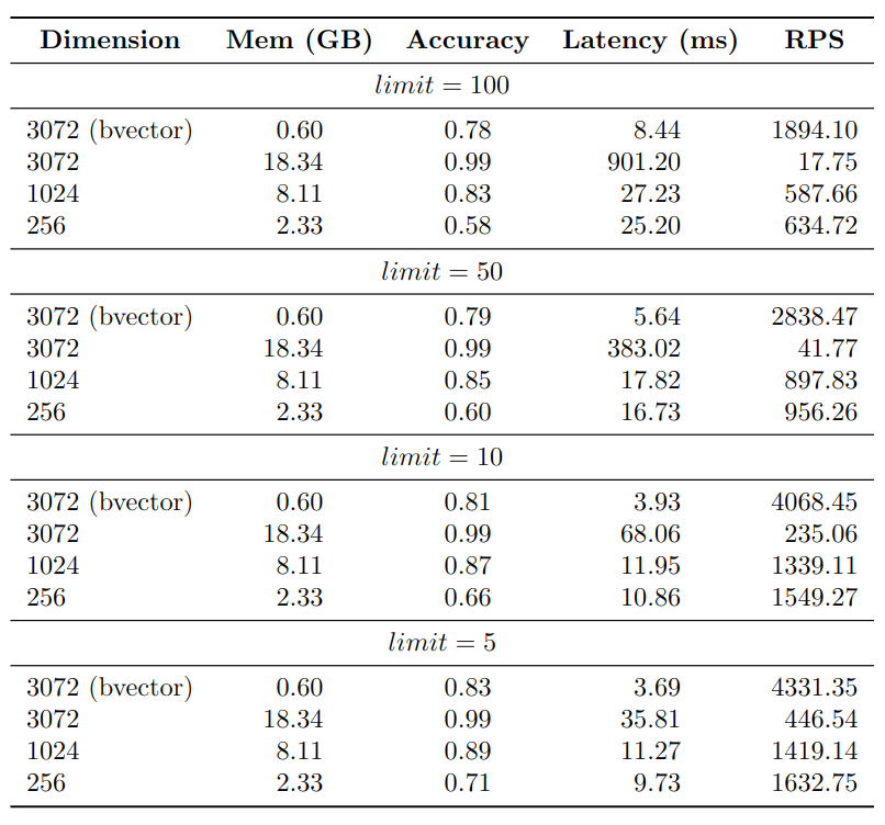
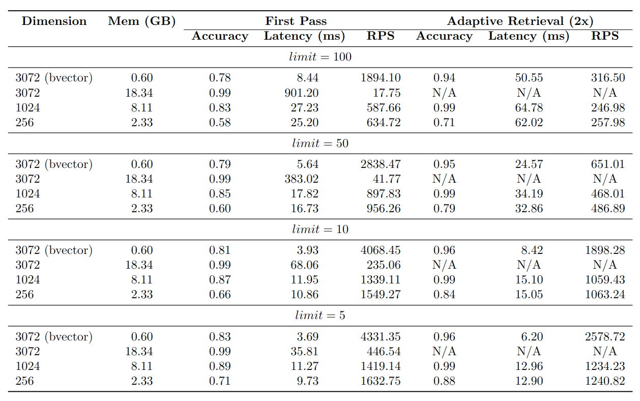
select id from openai3072 order by text_embedding_3_large_3072_embedding <-> (select text_embedding_3_large_3072_embedding from openai3072 where id = :random_id) limit 100;The results of the experiment are shown here:
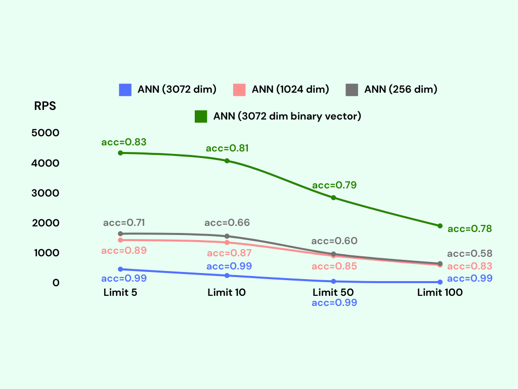
As anticipated, the 3072-dimensional embeddings exhibit the highest accuracy, while the 1024-dimensional embeddings demonstrate a slightly lower accuracy at around 85%. The 256-dimensional embeddings yield the lowest accuracy, approximately 65%. On the other hand, the binary vector index achieves an accuracy of about 80%.
Regarding the Requests Per Second (RPS) metric, the binary vector index showcases the most efficient performance, followed by the 256-dimensional embeddings, the 1024-dimensional embeddings, and finally, the 3072-dimensional embeddings.
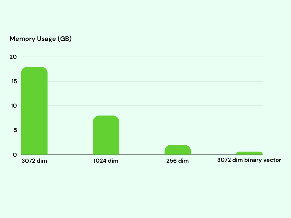
Details
The memory usage of the indexes is an important aspect to take into account. Indexing 1 million 3072-dimensional binary vectors requires only around 600MB of memory. In contrast, the 3072-dimensional vector index consumes approximately 18GB of memory. This represents a significant difference in memory usage, as the 3072-dimensional vector index utilizes approximately 30x more memory than the binary vector index.
Improve the accuracy via adaptive retrieval
Lower dimension and binary vector indexes trade off accuracy for advantages such as higher RPS and lower memory usage compared to full dimension indexes. Adaptive retrieval techniques can be used to combine the strengths of both approaches, achieving an optimized solution that balances accuracy, memory usage, and query speed.
The logic behind adaptive retrieval is really simple. Let's take get top 100 candidates as an example. We can perform the following steps:
- Query the lower dimensional or binary vector index first to retrieve 200 candidates from the 1 million embeddings. This is a fast operation.
- Rerank the candidates using a KNN query to retrieve the top 100 candidates. K-NN is well-suited for situations where smaller sets and precise similarity search are necessary, making it an excellent choice for reranking in this context.

The reranking step is a bit slower than the initial query, but it is still much faster than querying the full dimension index. It could be done in the pgvecto.rs:
CREATE OR REPLACE FUNCTION match_documents_adaptive(
  query_embedding vector(3072),
  match_count int
)
RETURNS SETOF openai3072
LANGUAGE SQL
AS $$
WITH shortlist AS (
  SELECT *
  FROM openai3072
  ORDER BY (text_embedding_3_large_3072_embedding[0:256])::vector(256) <-> (query_embedding[0:256])::vector(256)
  LIMIT match_count * 2
)
SELECT *
FROM shortlist
ORDER BY text_embedding_3_large_3072_embedding <-> query_embedding
LIMIT match_count;
$$;
The match_documents_adaptive function accepts a query embedding and a match count as input parameters. It first retrieves match_count * 2 candidates from the 1 million embeddings using the 256-dimensional index. Then, it reranks the candidates using a KNN query to retrieve the top match_count candidates.
The function for binary vector and 1024-dimensional embeddings can be implemented in a similar manner.
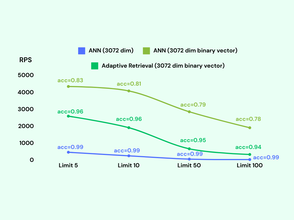
We conduct the benchmark again with the adaptive retrieval technique. We tag the adaptive retrieval technique as Adaptive Retrieval in the following figure.
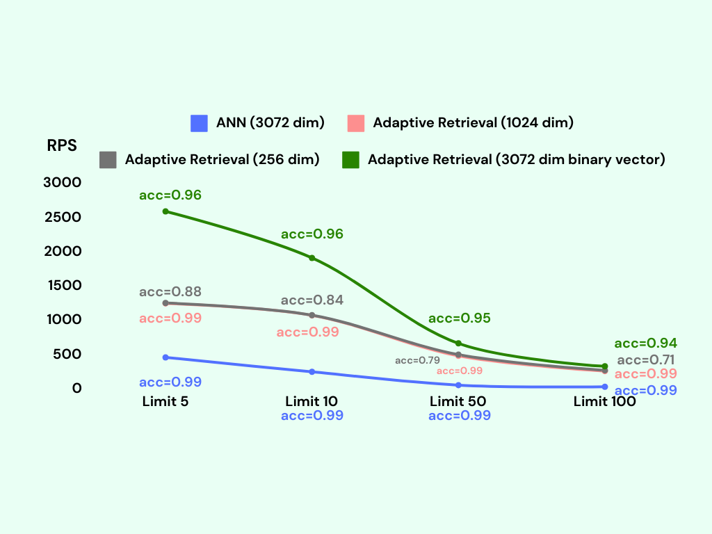
Adding a reranking step significantly improves the accuracy of the lower dimensional and binary vector indexes.
The binary vector index with adaptive retrieval achieves an accuracy of around 95%, with only a slight decrease in RPS compared to the binary vector index without adaptive retrieval. Remarkably, the memory usage of the binary vector index with adaptive retrieval is only around 600MB, which is the same as the binary vector index without adaptive retrieval.
Details
Conclusion
Shortening embeddings can reduce the memory usage to store the embeddings, and speed up indexing and search. However, the accuracy of the shortened embeddings is not as good as the full embeddings. That's why we need to use adaptive retrieval techniques to improve the accuracy of the lower dimensional indexes.
It seems that binary vector indexes with adaptive retrieval are the best choice for the text-embedding-3-large model. You could also consider 1024-dimensional indexes with adaptive retrieval if you need a higher accuracy (e.g. 99%).
PS: All the code and data used in this experiment are available in the pgvecto.rs-matryoshka-embeddings-benchmark.